Bring your data to live!

GreyCat is a programmable temporal graph database, made for efficient and flexible data processing at scale

Database system

Efficient storing and retrieval of relational, temporal and geographic data as a graph.

Object-Oriented Programming

Break free from the query chains and enjoy the flexibility of object-oriented data processing.

Data Analytics Stack

Integrated tools and libraries to identify and visualize crucial insights of your data

Install GreyCat for free

Documentation Install Introduction

Our community version is completely free

A Programable Database

All the benefits of a graph database without needing to learn a new fringe syntax.

No Query

No need for complex queries, traverse a graph as you would a simple object with dot notation.

No Mapping

A single Data Model from Disk to Api.

Any Scale

Datasets do not impose the infrastructure anymore, Hardware defines the speed.

No Tabular

No complex join or filters, leverage Object-Oriented traversal of the graph.

What If, Many Worlds

Simulate and store branches of your current state in a simple manner.

Stateful programming

Reduce the cost and time of processing by keeping the state and resume from where you left on the next iteration.

Script or serve

Use GreyCat as a stateful scripting solution or serve webapps (backend & frontend) from one executable.

How Does It Work ?

From input to insight in 3 simple steps

Example Data Source

This dataset represents sensor readings taken at various global locations, with each row capturing the following information:

Latitude and Longitude: Coordinates of the sensor location
Sensor ID: Unique identifier for each sensor
Timestamp: Unix timestamp representing the date and time of the reading
Humidity: Humidity levels in percentage
Temperature: Temperature values in degrees Celsius

latitude,longitude,sensor_id,timestamp,humidity,temperature
40.712776,-74.005974,S001,1694508300,65.2,22.5
34.052235,-118.243683,S002,1694508360,58.7,24.0
51.507351,-0.127758,S003,1694508420,72.1,18.3
48.856613,2.352222,S004,1694508480,69.0,19.6
35.689487,139.691711,S005,1694508540,55.5,23.8
55.755825,37.617298,S006,1694508600,60.4,16.9
-33.868820,151.209290,S007,1694508660,64.8,20.1
19.432608,-99.133209,S008,1694508720,62.3,21.7
52.520008,13.404954,S009,1694508780,68.9,17.4
-23.550520,-46.633308,S010,1694508840,59.1,25.3

type Sensor {
  id: String;
  values: nodeTime<Measurement>;
}
type Measurement {
  temperature: float;
  humidity: float;
}
type CsvEntry {
  position: geo;
  id: String;
  timestamp: time;
  humidity: float;
  temperature: float;
}
// global variable, serve as graph entry-point
var sensor_index: nodeGeo<Sensor>;

Step 1: Data Modeling

Sensor: This object holds the id of each sensor and a list of Measurement values associated with it.
Measurement: Contains two attributes, temperature and humidity, represented as floating-point values.
CsvEntry: Defines the structure of each CSV row, mapping columns to typed fields including position (geo), id (String), timestamp (time), humidity and temperature (float).
A global variable, sensor_index, is used as the entry point of the data graph. It organizes sensors by geographical location.

This structured data model enables efficient organization and retrieval of sensor data for further analysis and operations.

Step 2: Import

The import() function reads the CSV file located at "data.csv" using a CsvReader object.
In the CsvFormat object we only need to specify which column represents time, to automatically read the values as our internal native time type.
For each line of data, the code extracts geographical coordinates (latitude and longitude) and looks up the corresponding sensor in the sensor_index.
If the sensor doesn't exist, it creates a new Sensor object and associates it with the given location.
A new Measurement object is created from the CSV values for humidity and temperature, and it's stored in the sensor's values at the correct timestamp.

@expose
fn import() {
  var format = CsvFormat { header_lines: 1 };
  var cr = CsvReader<CsvEntry>{ path: "data.csv", format: format };

  while (cr.can_read()) {
    var entry = cr.read();

    var sensor = sensor_index.resolve(entry.position);
    if (sensor == null) {
      sensor = Sensor {
        id: entry.id,
        values: nodeTime<Measurement>{}
      };
      sensor_index.set(entry.position, sensor);
    }

    var measurement = Measurement {
      humidity: entry.humidity,
      temperature: entry.temperature
    };

    sensor.values.setAt(entry.timestamp, measurement);
  }
}

@expose
fn temperature_std(center: geo, radius: float, t: time): float? {
  var gaussian = Gaussian<float> {};

  var circle = GeoCircle { center: center, radius: radius };
  for (sensor_location, sensor in sensor_index) {
    if (circle.contains(sensor_location)) {
      gaussian.add(sensor.values.resolveAt(t)?.temperature);
    }
  }
  return gaussian.std();
}

Step 3: Spatial + Temporal Analysis

The temperature_std() function calculates the standard deviation of temperature readings within a specified geographic area and time:

The @expose keyword exposes the function as callable API over HTTP protocols
The function takes three parameters: a center location, a radius, and a time t.
A GeoCircle object is created to represent the defined geographic area.
For each sensor in the sensor_index, if its location falls within the circle, the temperature at the given time is added to a Gaussian object; representing the distribution.
Finally, the standard deviation of the temperatures within the circle at the given time, is returned.

GreyCat In Production

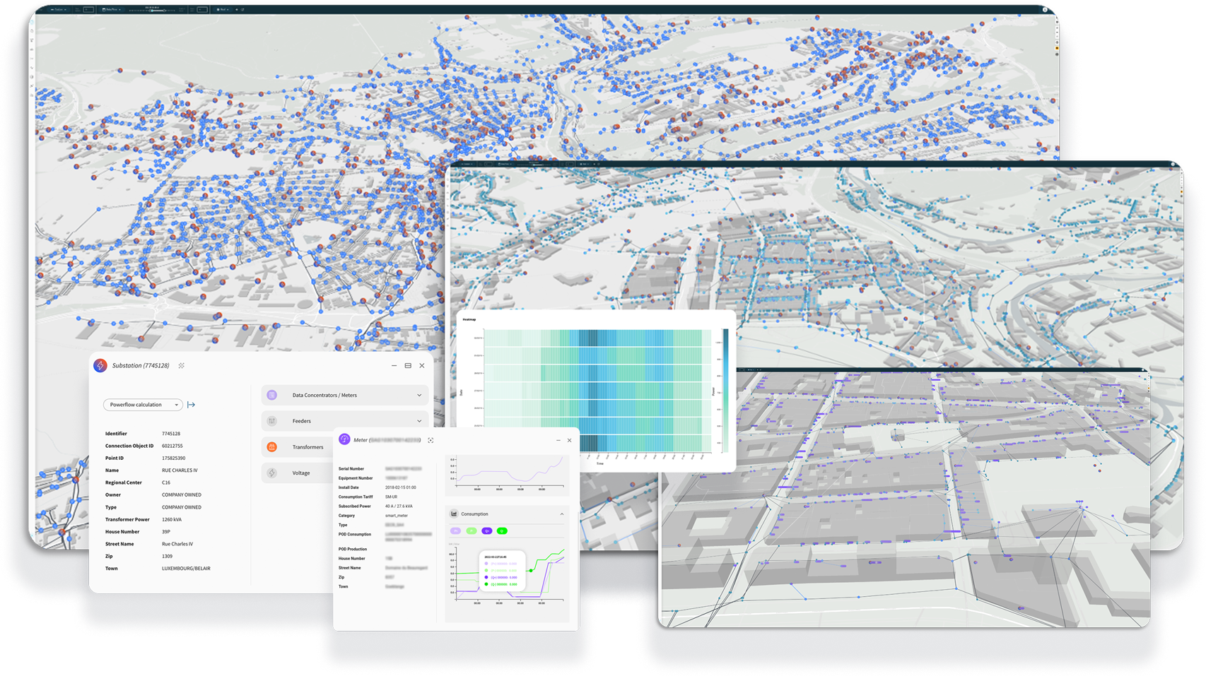
Kopr - Digital Twin

Kopr is a full-fledged AI Twin of the Luxembourg electricity grid. This digital counterpart of the physical grid and processes can be trained in near real-time – with the ever-increasing amount of available data – to serve as operational decision helper. Kopr aggregates, visualizes, analyzes, and learns data from various systems, e.g., GIS, SAP, metering infrastructures, real-time sensors, and much more. Kopr is built on top of our Greycat technology that allows us to scale to millions of grid elements and to billions of metering measurement points per year.

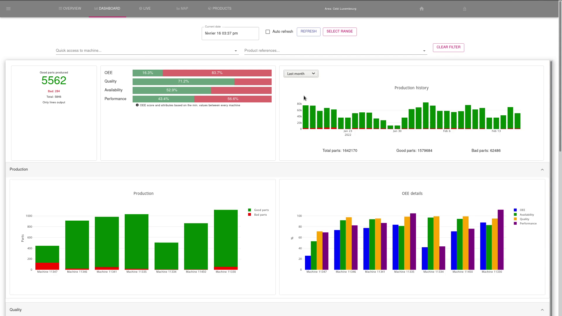
Predictive - Industry 4.0

To create a full scale digital twin of the factories, we used our core technology GreyCat to devise a suitable data structure to store and later analyze and learn from the production data with its context. Where possible, the existing connectivity of the production lines (PLCs) have been exploited to collect their data. In other places, made to measure sensors have been deployed (electricity, air pressure, temperature, vibration, etc.) to derive production indicators and detect anomalies.

Each production line (and each of its station/sensor/actuator) is profiled and monitored independently in live, enabling fine grained analysis and predictions of each of its composing elements. Learning from past experiences, algorithms are able to estimate the yields and provide insights on the evolution of the OEE. Using learned model, simulations can be run to estimate the impact of production plannings modification.

The history of GreyCat

From a theoretical idea into a fully fledged programming language managing & simulating an entire Countries energy grid

Learn more

Want to learn more about GreyCat ?

Our Blog Posts