The unified temporal-graph database for AI & digital twins
Time-series, graph, geo, vector and full-text search — unified in one self-hosted binary, with a built-in MCP server and on-device embeddings. No glue code, no sidecars.
curl -fsSL https://get.greycat.io/install.sh | bash -s stable
At a glance
Database system
Efficient storing and retrieval of relational, temporal and geographic data as a graph.
One language, disk to API
Model, store, and serve your data with a single object model — no ORM, no mapping layer.
Data Analytics Stack
Integrated tools and libraries to identify and visualize crucial insights of your data
Install GreyCat for free
Install Documentation IntroductionOur community version is completely free
Capabilities
Everything in one binary
GreyCat unifies five data systems — time-series, graph, geospatial, vector and full-text search — into a single ~4.6 MB engine with a built-in MCP server. Replace your polyglot stack with one self-hosted binary.
Time-series
Native temporal storage with point-in-time (as-of) queries and server-side sampling — no separate time-series database.
Graph
Traverse typed relationships with dot-notation — no JOINs and no separate query language to learn.
Geospatial
Native geo indexing and geometry, co-located with the rest of your data in the same store.
Vector search
A built-in vector index plus on-device embeddings — semantic search with no external embedding API.
Full-text search
BM25, hybrid and fuzzy search built in — no Elasticsearch sidecar to operate.
MCP server
A built-in Model Context Protocol server — your data and logic are AI-agent-ready out of the box.
Track record
Proven in production at scale
meter readings / year on a national electricity-grid digital twin
grid assets & 330k delivery points modelled live
searchable paragraphs in an enterprise legal-search platform
separate systems replaced by a single GreyCat binary
Consolidate
Replace your stack today
Most teams bolt together a time-series database, a graph database, a search cluster, a vector store, an embedding API and an MCP gateway — then pay to operate, sync and secure all of them. GreyCat does the same job in one self-hosted binary.
Compare GreyCat vs the polyglot stackYour stack today
Use cases
Built for AI & digital-twin workloads
One engine behind your most demanding temporal, graph and semantic workloads.
Go deeper
How GreyCat stacks up
An honest, side-by-side look at GreyCat next to the specialists — including the few places each incumbent still wins.
Compare side by sideFree to start, transparent editions
The Community edition is free forever. See what's included across Community, Pro and Enterprise.
View pricing & editionsDeveloper experience
A Programmable Database
All the benefits of a graph database without needing to learn a new fringe syntax.
No Query
No need for complex queries, traverse a graph as you would a simple object with dot notation.
No Mapping
A single Data Model from Disk to Api.
Any Scale
Datasets do not impose the infrastructure anymore, Hardware defines the speed.
No Tabular
No complex join or filters, leverage Object-Oriented traversal of the graph.
What-If, Many Worlds coming soon
Branch your data into parallel "what-if" worlds, simulate scenarios, and merge the results.
Stateful programming
Reduce the cost and time of processing by keeping the state and resume from where you left on the next iteration.
Script or serve
Use GreyCat as a stateful scripting solution or serve webapps (backend & frontend) from one executable.
AI-ready
Two annotations → a live API and an MCP tool
Write a function in GreyCat's
language. Add @expose and @tag and it is instantly a typed REST endpoint
and a Model Context Protocol tool your AI agents can call — no glue code, no separate gateway.
On the backend
Write a function & add two annotations…
@expose
@tag("openapi", "mcp")
fn add(a: int, b: int): int { return a + b; }@expose— turns the function into a typed REST endpoint@tag("openapi", "mcp")— adds it to the OpenAPI spec and the built-in MCP server- Same function, same RBAC — no controllers, DTOs or gateway to maintain
From the frontend & AI agents
Call it over HTTP like any REST endpoint…
curl -s https://your-server/add -d '[40, 2]'
# => 42
…or let an AI agent discover and run it over MCP:
initialize— the agent connects to GreyCat's built-in MCP servertools/list—addappears automatically with its typed schematools/call— the agent invokes it, under the same RBAC as every caller
Case studies
GreyCat In Production
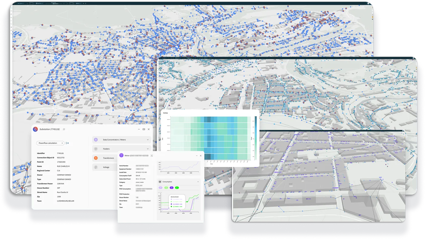
Kopr - Digital Twin
Kopr is a full-fledged AI Twin of the Luxembourg electricity grid. This digital counterpart of the physical grid and processes can be trained in near real-time – with the ever-increasing amount of available data – to serve as operational decision helper. Kopr aggregates, visualizes, analyzes, and learns data from various systems, e.g., GIS, SAP, metering infrastructures, real-time sensors, and much more. Kopr is built on top of our GreyCat technology that allows us to scale to millions of grid elements and to billions of metering measurement points per year.
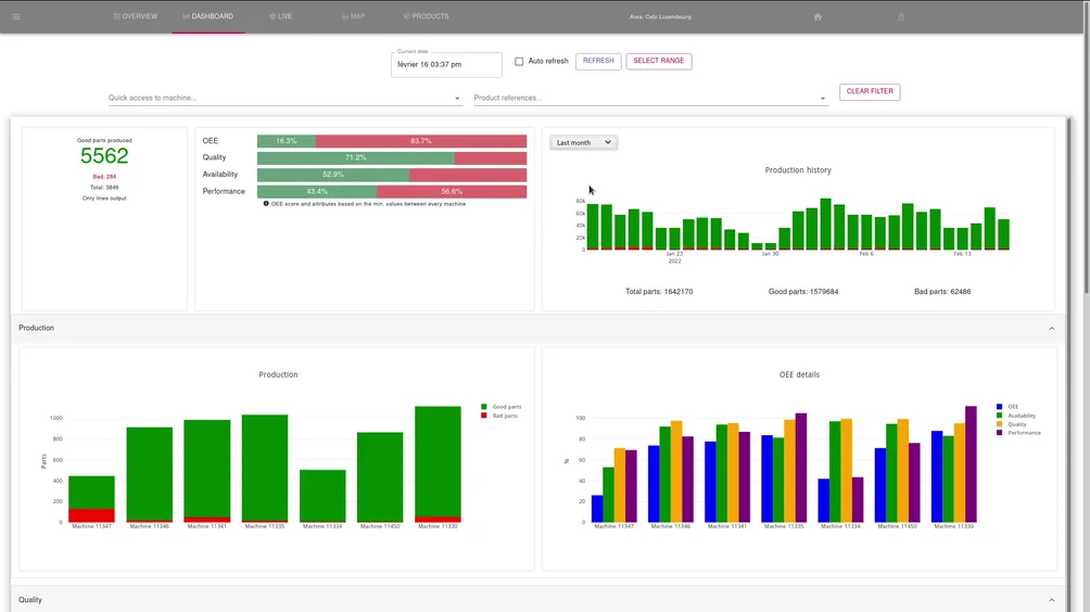
Predictive - Industry 4.0
To create a full scale digital twin of the factories, we used our core technology GreyCat to devise a suitable data structure to store and later analyze and learn from the production data with its context. Where possible, the existing connectivity of the production lines (PLCs) have been exploited to collect their data. In other places, made to measure sensors have been deployed (electricity, air pressure, temperature, vibration, etc.) to derive production indicators and detect anomalies.
Each production line (and each of its station/sensor/actuator) is profiled and monitored independently in live, enabling fine grained analysis and predictions of each of its composing elements. Learning from past experiences, algorithms are able to estimate the yields and provide insights on the evolution of the OEE. Using learned model, simulations can be run to estimate the impact of production plannings modification.
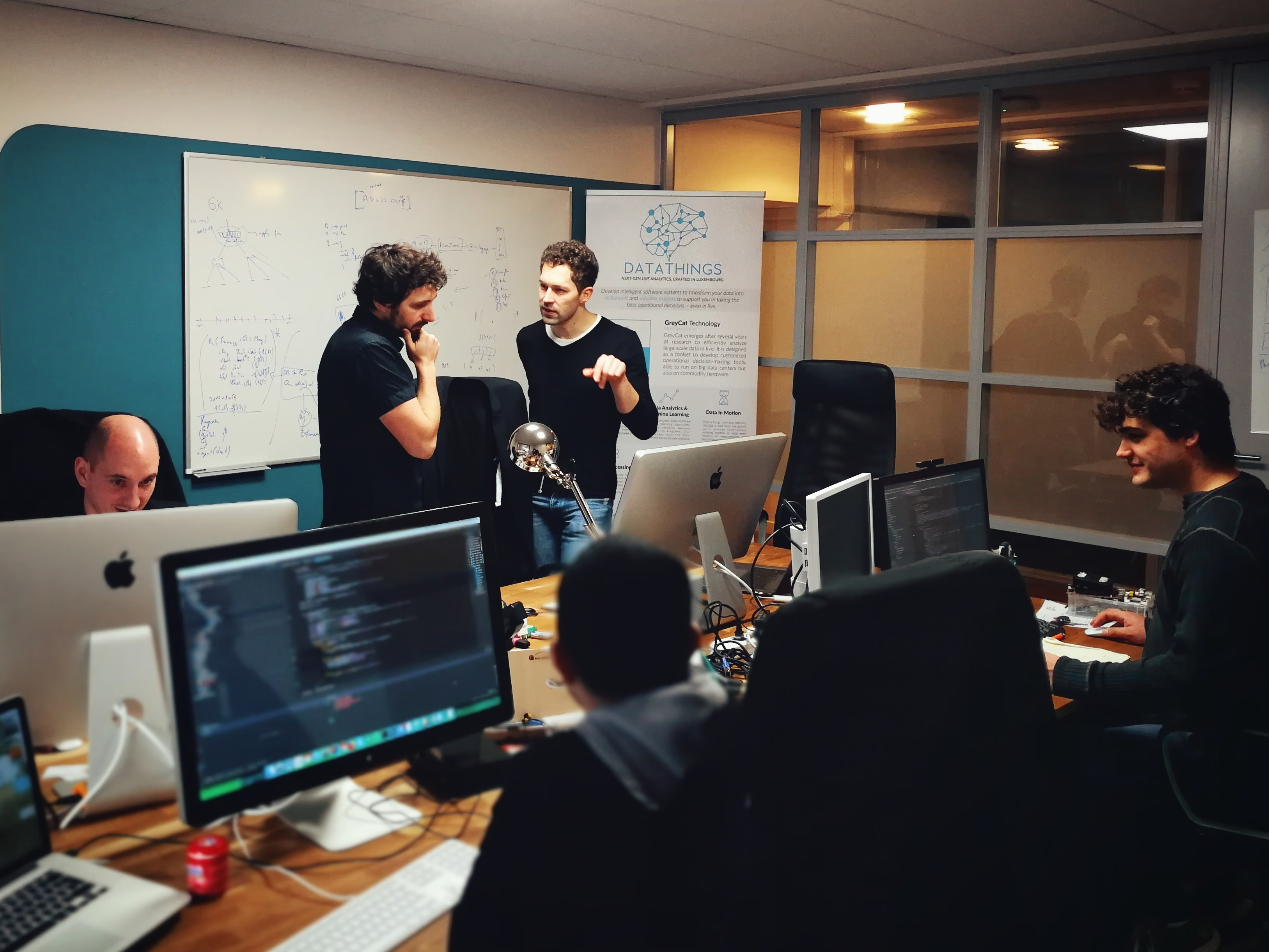
Our story
The history of GreyCat
From a theoretical idea into a fully fledged programming language managing & simulating an entire country's energy grid
Learn more about our historyWant to learn more about GreyCat?
Our Blog Posts
Get started
Start building in a unified tech stack
Install the free Community edition in seconds, or talk to us about Pro and Enterprise.